Chapter 6 Using R Markdown

Before going into more details of R Markdown, let’s talk about two common options in the world of R coding: the R script (.R) and the dynamic R Markdown document (.Rmd).

R Scripts: Imagine coding as crafting a detailed recipe of R commands—a script—that guides R through specific tasks. Conventional R scripts (.R files) are dedicated to these commands, handling calculations and operations. However, as scripts grow, they become complex and sharing insights alongside code becomes challenging.

R Markdown: R Markdown (.Rmd) elevates the coding experience by harmonizing code with explanatory text. Within an R Markdown document, code blocks act like individual scripts—smaller, more focused units. These blocks merge code with explanations seamlessly, creating a coherent narrative. Unlike isolated scripts, R Markdown emphasizes both code functionality and its significance within the context. For these reasons, we’ll be sticking to working in .Rmd files.

In a nutshell, R Markdown allows you to analyse your data with R and write your report in the same place (this entire book was written with R Markdown). This has loads of benefits including a reproducible workflow, and streamlined thinking. No more flipping back and forth between coding and writing to figure out what’s going on.

Let’s run some simple code as an example:

x <- 2+2
x

## [1] 4

What we’ve done here is write a snippet of R code, ran it, and printed the results (as they would appear in the console). While the above code isn’t anything special, we can extend this concept so that our R markdown document contains any data, figures or plots we generate throughout our analysis in R. For example:

library(tidyverse) 
library(knitr)

airPol <- read_csv("data/2018-01-01_60430_Toronto_ON.csv")

ggplot(data = airPol, 
       aes(x = date.time, 
           y = concentration, 
           colour = pollutant)) + 
  geom_line() +
  theme_classic()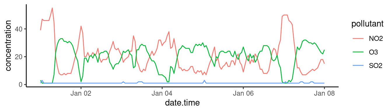

Time series of 2018 ambient atmospheric O~3~, NO~2~, and SO~2~ concentrations (ppb) in downtown Toronto

Figure 6.1: Time series of 2018 ambient atmospheric O₃, NO₂, and SO₂ concentrations (ppb) in downtown Toronto

sumAirPol <- airPol %>%
  drop_na() %>%
  group_by(city, naps, pollutant) %>%
  summarize(mean = mean(concentration), 
            sd = sd(concentration), 
            min = min(concentration), 
            max = max(concentration))

knitr::kable(sumAirPol, digits = 1)

city	naps	pollutant	mean	sd	min	max
Toronto	60430	NO2	20.5	11.5	7	55
Toronto	60430	O3	19.7	8.7	1	33
Toronto	60430	SO2	1.1	0.3	1	3

Pretty neat, eh? You might not think so, but let’s imagine a scenario you’ll encounter soon enough. You’re about to submit your assignment, you’ve spent hours analyzing your data and beautifying your plots. Everything is good to go until you notice at the last minute you were supposed to subtract value x and not value y in your analysis. If you did all your work in Excel (tsk tsk), you’ll need to find the correct worksheet, apply the changes, reformat your plots, and import them into word (assuming everything is going well, which it never does with looming deadlines). Now if you did all your work in R markdown, you go to your one .rmd document, briefly apply the changes and re-compile your document.

A lot of scientists work with R Markdown for writing their reports for numerous reasons:

Integrated Workflow: Combines narrative, data analyses, and visualizations in one document, promoting reproducibility and transparency.
Versatility: Easily exports to diverse formats like HTML, PDF, and Word, catering to different dissemination needs.
Plot Management: Offers precise control over visual presentations, allowing for tailored figure sizes, resolutions, and formats.

In sum, R Markdown provides a streamlined platform for scientific communication, merging data analysis with polished publication seamlessly.

6.1 Getting started with R Markdown

As you’ve already guessed, R markdown documents use R and are most easily written and assembled in RStudio. If you have not done so, revisit Chapter 1:[Installing R]. Once setup with R and R Studio, you’ll need to install the R Markdown and tinytex packages by running the following code in the console:

# These are large packages so it'll take a couple of minutes to install

install.packages("R Markdown") # downloaded from CRAN

install.packages("tinytex")
tinytex::install_tinytex()  # install TinyTeX

The R Markdown package is what we’ll use to generate our documents, and the tinytex package enables compiling documents as PDFs. There’s a lot more going on behind the scenes, but you shouldn’t need to worry about it.

Now that everything is setup, you can create your first R Markdown document by opening up R Studio, selecting FILE -> NEW FILE -> R Markdown. A dialog box will appear asking for some basic input parameters for your R markdown document. Add your title and select PDF as your default output format (you can always change these later if you want). A new file should appear that’s already populated with some basic script illustrating the key components of an R markdown document.

6.1.1 Understanding R Markdown

Your first reaction when you opened your newly created R markdown document is probably that it doesn’t look anything at all like something you’d show your prof. You’re right, what you’re seeing is the plain text code which needs to be compiled (called knit in R Studio) to create the final document. When you create a R markdown document like this in R Studio a bunch of example code is already written. You can compile this document (see below) to see what it looks like, but let’s break down the primary components. At the top of the document you’ll see something that looks like this:

---
title: "Temporal Analysis of Foot Impacts While Birling Down the White Water"
author: "Jean Guy Rubberboots"
date: "24/06/2021"
output: pdf_document
---

This section is known as the preamble and it’s where you specify most of the document parameters. In the example we can see that the document title is “Temporal Analysis of Foot Impacts While Birling Down the White Water”, it’s written by Jean Guy Rubberboots, on the 24th of June, and the default output is a PDF document. You can modify the preamble to suit your needs. For example, if you wanted to change the title you would write title: "Your Title Here" in the preamble. Note that none of this is R code, rather it’s YAML, the syntax for the document’s metadata. Apart from what’s shown you shouldn’t need to worry about this much, just remember that indentation in YAML matters.

6.1.1.1 Output Options in R Markdown

You can compile your entire document using the Knit document button. This is a great way to tinker with your code before you compile your document. Knitting will sequentially run all of your code chunks, generate all the text, knit the two together and output a PDF. You’ll basically save this for the end.

R Markdown offers flexibility in terms of output formats, allowing users to knit their documents into various outputs tailored to their needs.

Three Common Output Options:

HTML (html_document): Produces an HTML file, suitable for hosting on websites or for sharing via email. This format allows for interactive content, making it ideal for interactive graphs or web applications.
PDF (pdf_document): Creates a PDF file. This format is best for documents intended for print or formal submissions, as it maintains consistent formatting across different devices and platforms.
Word (word_document): Generates a Microsoft Word document, which can be useful when sharing drafts or collaborating with colleagues who use Word for edits.

Controlling the Output:

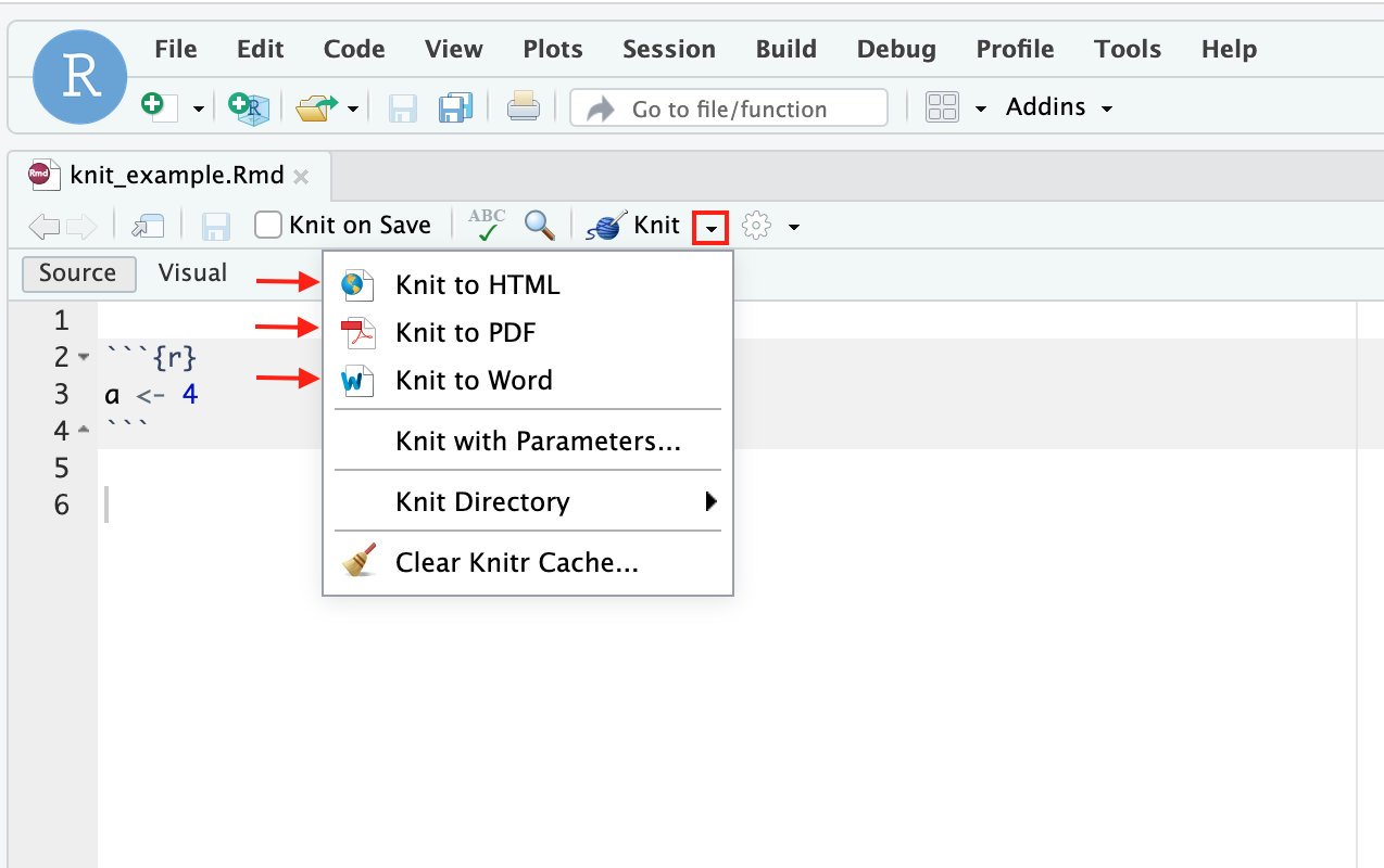
Modifying the YAML Header: You can change the output format directly in the YAML header of your Rmd file. In the last example, replacing output: pdf_document with output: html_document or output: word_document would knit the document into HTML or Word, respectively.
Using RStudio’s Knit Button: In the RStudio IDE, at the top of the script editor pane, there’s a Knit button. Clicking the small dropdown arrow next to this button allows you to choose the output format you desire. Selecting one of the options will knit the document into that format and update the YAML header accordingly.

6.1.2 Running code in R Markdown

6.1.2.1 How to create code chunks

To create a code chunk within RStudio, you have several options:

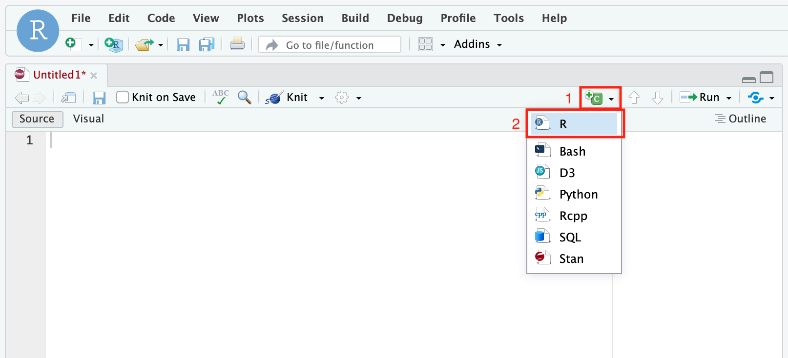
Use the green “c” button located at the top right corner of your file view and select “R”. Make sure your cursor is positioned at the desired location within your .rmd file when you do this.

Type ```{r} – three back-ticks followed by {r} – to initiate a new code chunk, and type ``` – three backticks (```) – to end the code chunk. You can specify code chunks options in the curly braces. i.e. ```{r, fig.height = 2} sets figure height to 2 inches. See the Code Chunk Options section below for more details.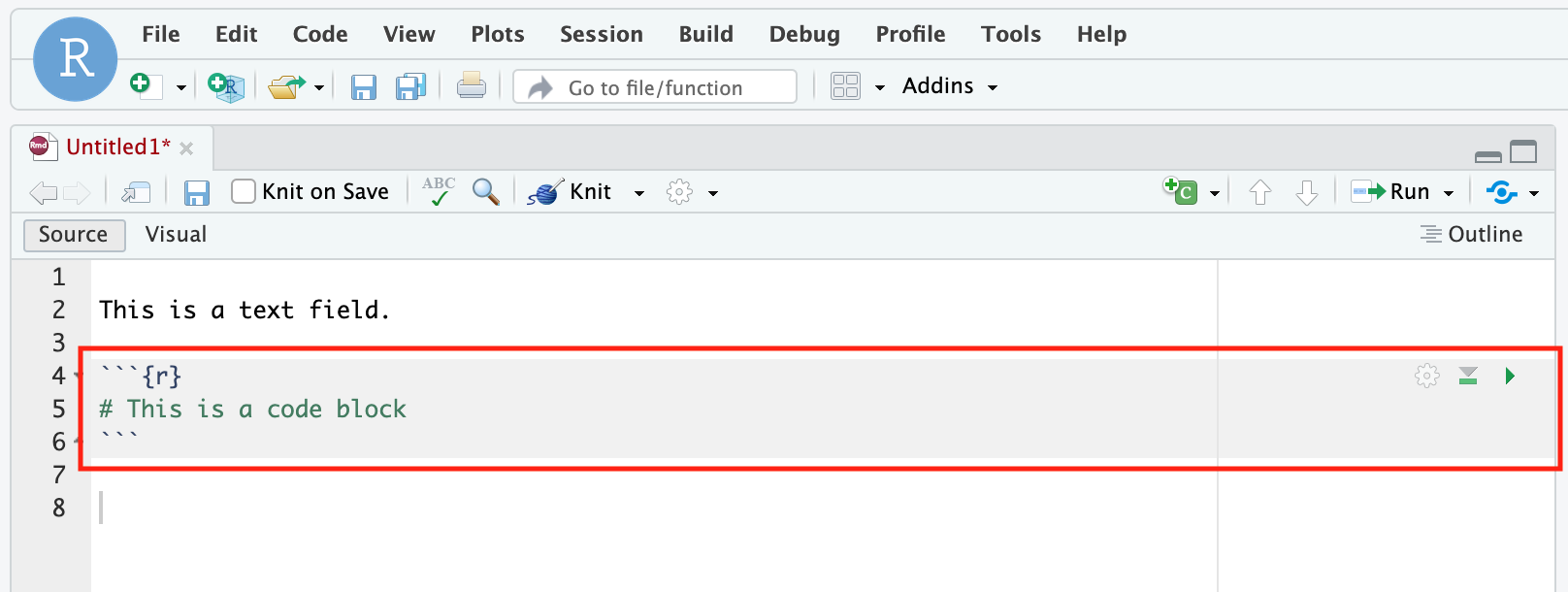

Inline code expression, which starts with `r and ends with ` in the body text. Earlier we calculated x <- 2 + 2, we can use inline expressions to recall that value.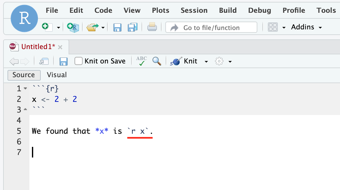

When we knit the markdown file shown in the figure, the knitted document will say “We found that x is 4.”

6.1.2.2 How to run code chunks

To run code within an R Markdown document, you again have various options to choose from.

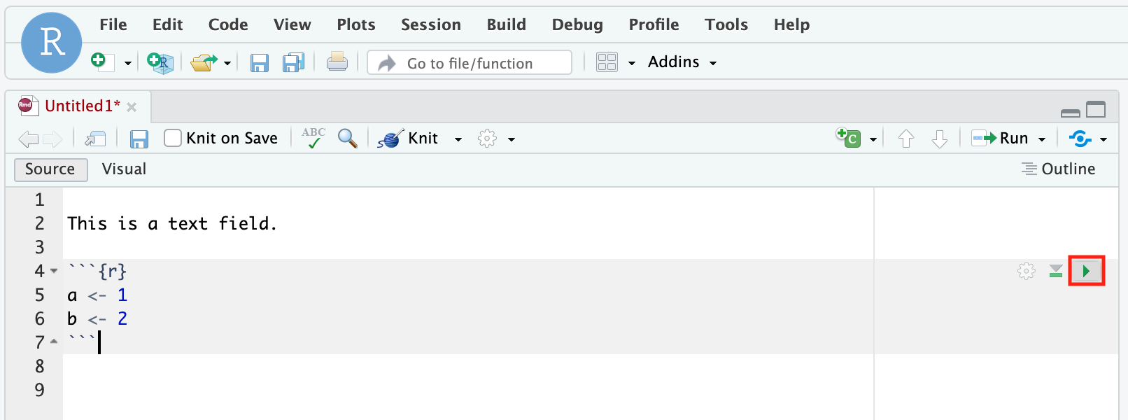
You can run a specific code chunk by clicking the green triangle button located within each chunk. This action will execute the entire chunk, including all the code it contains.

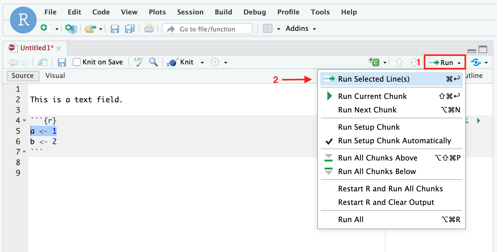
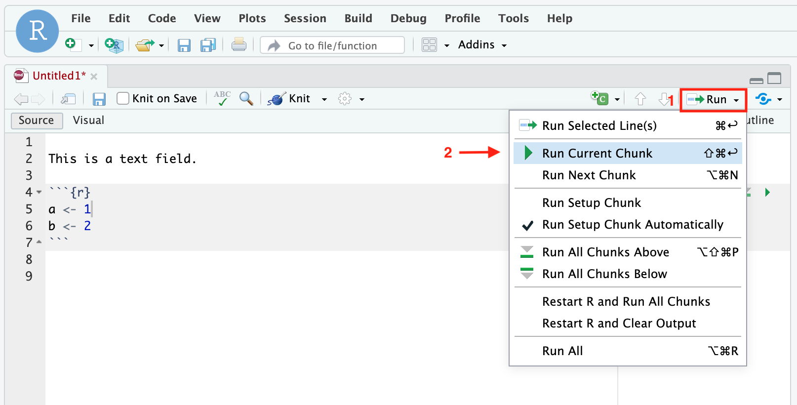
Run a code chunk using its own run button.

For more control, you can run selected lines or chunks. To do this, use the “Run” button at the top of the file view. This button provides a range of execution options that allow you to run code in a manner that suits your needs.

Example: Run selected line(s)

Example: Run Current Chunk

Note all the code chunks in a single markdown document work together like a normal R script. That is if you assign a value to a variable in the first chunk, you can call this variable in the second chunk; the same applies for libraries. Also note that every time you compile a markdown document, it’s done in a “fresh” R session. If you’re calling a variable that exist in your working environment, but isn’t explicitly created in the markdown document you’ll get an error.

6.1.3 Headings and Subheadings

In R Markdown, structuring your document with clear headings and subheadings is simple using the pound (#) sign. This not only helps in organizing content but also aids in creating a table of contents if required.

Main Headings: Use a single pound sign (i.e. # Main Heading)
Subheadings: Increase the number of pound signs based on the level of the subheading.
- ## Subheading Level 1
- ### Subheading Level 2
- #### Subheading Level 3

R Markdown will automatically format these appropriately when the document is knit. For example, a main heading will typically appear larger and bolder than its subheadings, like this:

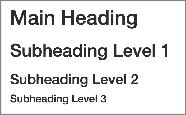
By effectively utilizing headings and subheadings, you can provide clear structure and flow to your document, making it more readable and navigable for your audience.

6.1.4 LaTeX Basics

LaTeX (pronounced “Lay-tech”) is a typesetting system that’s popular in academia due to its high-quality output format and the ability to handle complex formatting tasks. It’s especially favored for documents that contain mathematical symbols, equations, and other specialized notation.

In R Markdown, LaTeX code can be integrated directly into your document to allow for advanced formatting, especially for mathematical expressions and equations. When you knit your R Markdown document, the LaTeX code is rendered into beautifully formatted text.

There are two common ways to turn your expressions in a math mode.

Display mathematical expressions: centers the mathematical expression on its own line
Inline mathematical expressions: appears within the flow of a sentence or text

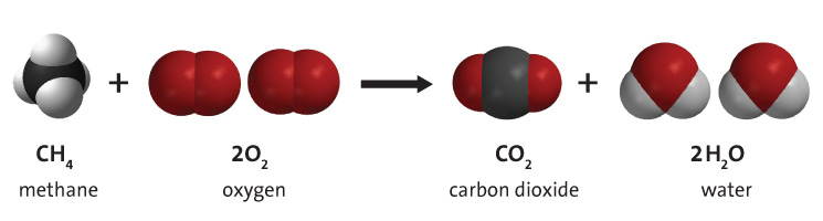
For chemistry students, one common use of LaTeX is to typeset chemical equations. We will provide examples on the combustion of methane:

6.1.4.1 Display math mode

You can have an entire line in a math mode using either \[...\] or $$...$$.

When you write it in rmd, it would look like :

\[ \text{CH}_4 + 2\text{O}_2 \rightarrow \text{CO}_2 + 2\text{H}_2\text{O} \] or $$ \text{CH}_4 + 2\text{O}_2 \rightarrow \text{CO}_2 + 2\text{H}_2\text{O} $$

When you knit it, it will be displayed as:
\[ \text{CH}_4 + 2\text{O}_2 \rightarrow \text{CO}_2 + 2\text{H}_2\text{O} \]

6.1.4.2 Inline math mode

On the other hand, if you want to insert your expression within your sentence, you can use $...$ syntax.

With our methane combustion example, we can write something like this:

Methane ($\text{CH}_4$) reacts with oxygen ($\text{O}_2$) to produce carbon dioxide ($\text{CO}_2$) and water ($\text{H}_2\text{O}$).

When you knit it, this will be displayed as:

Methane ($\text{CH}_4$) reacts with oxygen ($\text{O}_2$) to produce carbon dioxide ($\text{CO}_2$) and water ($\text{H}_2\text{O}$).

6.1.4.3 Useful LaTeX Syntax

Now that you’ve seen how you can write your scientific expression in two different ways, let’s look at some useful LaTeX Syntax for our purpose.

Symbols
- Greek letters: Use a backslash followed by the name of the letter, e.g., \alpha for $\alpha$.
- Special symbols
  - \times for $\times$
  - \approx for $\approx$
  - \geq for $\geq$
  - \rightarrow for $\rightarrow$
Superscripts and Subscripts
- Superscripts: x^2 renders as $x^2$.
- Subscripts: H_2O renders as $H_2O$
Formatting
- Boldface: \textbf{Text} for $\textbf{Text}$
- Italics: \textit{Text} for $\textit{Text}$

In R Markdown, you can place your cursor over a LaTeX expression to preview its rendered output. This allows you to verify that the LaTeX formatting is correct before knitting the document.

6.1.4.4 More LaTeX Resources

There are numerous online resources dedicated to LaTeX symbols and their usage.

A popular starting point is the Comprehensive LaTeX Symbol List, available on CTAN (Comprehensive TeX Archive Network). This extensive compilation offers a wide range of symbols used in various disciplines.
Additionally, platforms like Detexify allow users to sketch a symbol, and the tool then identifies the corresponding LaTeX command.
Engaging with online communities, such as the TeX - LaTeX Stack Exchange, can also be invaluable for finding specific symbols or seeking advice on LaTeX-related challenges.

6.2 Compiling your final report

To create a PDF to hand in, you’ll need to compile, or knit, your entire markdown document as mentioned above. To knit your R markdown script, simply click the knit button in R Studio (yellow box, Figure 2). You can specify what output you would like and R Studio will (hopefully) compile your script. Remember, you can test or run individual code chunks as outlined in Running code in R Markdown.

6.3 Authoring with R Markdown

Below is a brief summary of the major elements required to author an R Markdown document. They should address the majority of your needs, but please see the R Markdown resources for more information.

6.3.1 R markdown syntax

Unlike Microsoft Word, R Markdown utilizes a specific syntax for text formatting. Once you get used to it, it makes typing documents much easier than Word’s approach. The table below is how some of the most common text formatting is typed in your R Markdown document (syntax & example column) and how it’ll appear in the final output.

Text formatting	syntax	Example	Example output
italics	text	this is italics	this is italics
bold	text	this is bold	this is bold
subscript	~text~	this is ~subscript~	this is _subscript
superscript	^text^	this is ^superscript^	this is ^superscript
monospace	`text`	this is `monospaced`	this is `monospace`

For a collection of other R Markdown syntax, please see the useful (and brief) list compiled online here. This includes ordered and unordered lists, headers, code blocks, hyperlinks, and figure captions.

6.3.2 R code chunk options

Your R code is run in chunks and the results will be embedded in the final output file. To each chunk you can specify options that’ll affect how your code chunk is run and displayed in the final output document. You include options in the chunk delimiters ```{r} and ```. For example the following code tells markdown you’re running code written in R, that when you compile your document this code chunk should be evaluated, and that the resulting figure should have the caption “Some Caption”.

```{r, eval = FALSE, fig.cap = "Some caption"}

# some code to generate a plot worth captioning. 

```

The most common and useful chunk options are shown below. Note that they all have a default value. For example, eval tells R markdown whether the code within the block should be run. It’s default option is TRUE, so by default any code in a chunk will be run when you knit your document. If you don’t want that code to be run, but still displayed, you would set eval = FALSE. Another example would be setting echo = FALSE which allows the code to run, but the code won’t be displayed on the output document (the outputs will still be displayed though); useful for creating clean documents with plots only (i.e. lab reports…).

option	default	effect
eval	TRUE	whether to evaluate the code and include the results
echo	TRUE	whether to display the code along with its results
warning	TRUE	whether to display warnings
error	FALSE	whether to display errors
message	TRUE	whether to display messages
tidy	FALSE	whether to reformat code in a tidy way when displaying it
fig.width	7	width in inches for plots created in chunk
fig.height	7	height in inches for plots created in chunk
fig.cap	NA	include figure caption, must be in quotation makrs (““)

6.3.3 Inserting images

Images not produced by R code can easily be inserted into your document. The markdown code isn’t R code, so between paragraphs of bodytext insert the following code.

![Caption for the picture.](path/to/image.png){width=50%, height=50%}

Note that in the above the use of image attributes, the {width=50%, height=50%} at the end. This is how you’ll adjust the size of your image. Other dimensions you can use include px, cm, mm, in, inch, and %.

A final note on images: when compiling to PDF, the LaTeX call will place your image in the “optimal” location (as determined by LaTeX), so you might find your image isn’t exactly where you thought it would be. A more in-depth guide to image placement can be found here

6.3.4 Generating tables

There are multiple methods to create tables in R markdown. Assuming you want to display results calculated through R code, you can use the kable() function. Or you can consult the Summarizing Data chapter for making publication ready tables.

Alternatively, if you want to create simple tables manually use the following code in the main body, outside of an R code chunk. You can increase the number of rows/columns and the location of the horizontal lines. To generate more complex tables, see the kable() function and the kableExtra package.

Header 1 | Header 2| Header 3
---------|---------|---------|
Row 1    | Data    | Some other Data
Row 2    | Data    | Some other Data
---------|---------|---------|

Header 1	Header 2	Header 3
Row 1	Data	Some other Data
Row 2	Data	Some other Data

We know this can be a tedious process. Luckily, there is a website that generates the markdown syntax when you input the values, and this can save your time trying to correctly format tables. Check it out here.

6.3.5 Spellcheck in R Markdown

While writing an R markdown document in R studio, go to the Edit tab at the top of the window and select Check Spelling. You can also use the F7 key as a shortcut. The spell checker will literally go through every word it thinks you’ve misspelled in your document. You can add words to it so your spell checker’s utility grows as you use it. Note that the spell check may also check your R code; be wary of changing words in your code chunks because you may get an error down the line.

6.3.6 Exporting R Markdown documents

You’ll most likely be exporting your R Markdown documents as PDFs, but the beauty of R Markdown is it doesn’t stop there. Your R Markdown documents can be knitted as a HTML document, a book (or both like this book!). You can even make slideshow presentations and yes, if need be, export as a word document that you can open in Microsoft Word.

You specify the output format in the document header. To specify you want your document to be outputted as a PDF your YAML header would look like this:

---
title: "Your title here"
output: pdf_document
---

Here are some links to different output formation available in R Markdown and how to use them:

pdf_document creates a PDF document via Latex; probably your defacto output.
word_document creates a Word document. Note that the formatting options are pretty basic, so while everything will be where you want it to be, you’ll need to pretty it up in Word to comply with your instructor’s specifications.
tufte_handout for a PDF handout in the style of Edward Tufte. Check it out.
ioslides_presentation, revealjs::revealjs_presentation, and powerpoint_presentation are all options to create slideshow presentations. I personally use revealjs for my own work. It has the steepest learning curve of the bunch, but once setup, you can make incredibly slick slides with ease.
- Note: like word_document, powerpoint_presentation’s outputs are stylistically simple. You’ll definitely need to pretty them up manually in Powerpoint.

6.3.7 RStudio tips and tricks

To further the usefulness of R Markdown, the latest release of RStudio has a Visual R Markdown editor which introduces many useful features for authoring documents in R Markdown. Some of the most pertinent are:

Visual editor so you can see how your document looks (top left of script pane)
Combining Zotero and RStudio for easy citations, of your document (read more here)

6.4 R Markdown resources

There’s a plethora of helpful online resources to help hone your R markdown skills. We’ll list a couple below (the titles are links to the corresponding document):

Chapter 2 of the R Markdown: The Definitive Guide by Xie, Allaire & Grolemund (2020). This is the simplest, most comprehensive, guide to learning R markdown and it’s available freely online.
The R markdown cheat sheet, a great resource with the most common R markdown operations; keep on hand for quick referencing.
Bookdown: Authoring Books and Technical Documents with R Markdown (2020) by Yihui Xie. Explains the bookdown package which greatly expands the capabilities of R markdown. For example, the table of contents of this document is created with bookdown.