Chapter 15 Restructuring Your Data

In the realm of data analysis, the structure of your data can be just as crucial as the data itself. When dealing with complex datasets in R, or any other analytical environment, the way you organize and reshape your data can significantly impact the efficiency and clarity of your analyses. This chapter delves into the art of restructuring data in R, focusing on two powerful tidyverse functions: pivot_longer and pivot_wider. These tools are essential for transforming data into a format that aligns perfectly with your analytical objectives.

Understanding and mastering these functions will equip you with the skills to seamlessly toggle between different data layouts. Whether you need to condense wide datasets into longer, more detailed formats using pivot_longer, or expand long datasets into a wider, more summarized form with pivot_wider, this chapter will guide you through each step with practical examples and insights. By the end of this chapter, you’ll not only be adept at manipulating your data’s structure in R but also appreciate how such transformations can unveil new perspectives and insights in your data analysis journey.

15.1 Long vs Wide Data

Let’s revisit our ATR plastics data from previous chapters:

atr_plastics <- read.csv("data/ATR_plastics.csv")

DT::datatable(head(atr_plastics, 50))

And here is the surprise: The data you see above was actually already transformed to be longer for your convenience in the earlier chapters!

The original (wide) data looks like this:

atr_plastics_wide <- read.csv("data/ATR_plastics_original_wide.csv")

# This just outputs a table you can explore within your browser
DT::datatable(atr_plastics_wide)

15.1.1 Long Data

In the long format, the data is structured with each observation occupying a single row, and different variables are stacked or melted into a single column.

Take a look at the data atr_plastics. It contains absorbance measurements for different materials (EPDM, Polystyrene, Polyethylene, and a sample labeled “Sample: Shopping bag”) at various wavenumbers. Each row represents a combination of wavenumber, material, and absorbance value. This format is more conducive to data analysis and visualization, particularly when working with multiple variables or when conducting statistical analyses. It allows for easier manipulation and transformation of the data, as well as the application of statistical models that require data in long format, such as certain regression analyses. This is exactly why we have been providing you with this version of data in the previous chapters!

15.1.2 Wide Data

On the other hand, in the wide format, the data (atr_plastics_wide) is organized with each variable occupying its own column. Here, we have a dataset containing the same absorbance measurements, but now each row represents a unique wavenumber, and the absorbance values for each material are presented in separate columns. This format is intuitive for viewing all measurements at a particular wavenumber simultaneously, allowing for quick comparisons between materials.

However, as the number of materials or variables increases, the wide format may become unwieldy, especially if additional variables are introduced.

This format makes intuitive sense when recording in the lab, and for working in Excel, but isn’t the friendliest with R. For example, when making plots with ggplot, we can only specify one y variable. In the example plot below it’s the absorbance spectrum of Polystyrene. However, if wanted to plot the other spectra for comparison, we’d need to repeat our geom_point call for each variable, which is not ideal to keep our code clean.

# Plotting Polystyrene absorbance spectra
ggplot(data = atr_plastics_wide, 
       aes( x = wavenumber,
            y = Polystyrene)) +
  geom_point()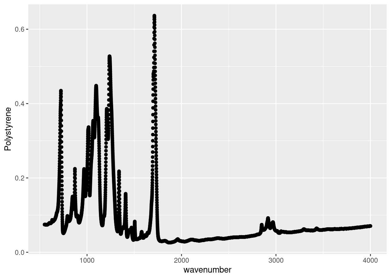

# Plotting Polystyrene and Polyethylene absorbance spectra
ggplot(data = atr_plastics_wide, 
       aes(x = wavenumber,
           y = Polystyrene)) +
  geom_point() +
  geom_point(data = atr_plastics_wide, 
             aes(x = wavenumber, 
                 y = Polyethylene))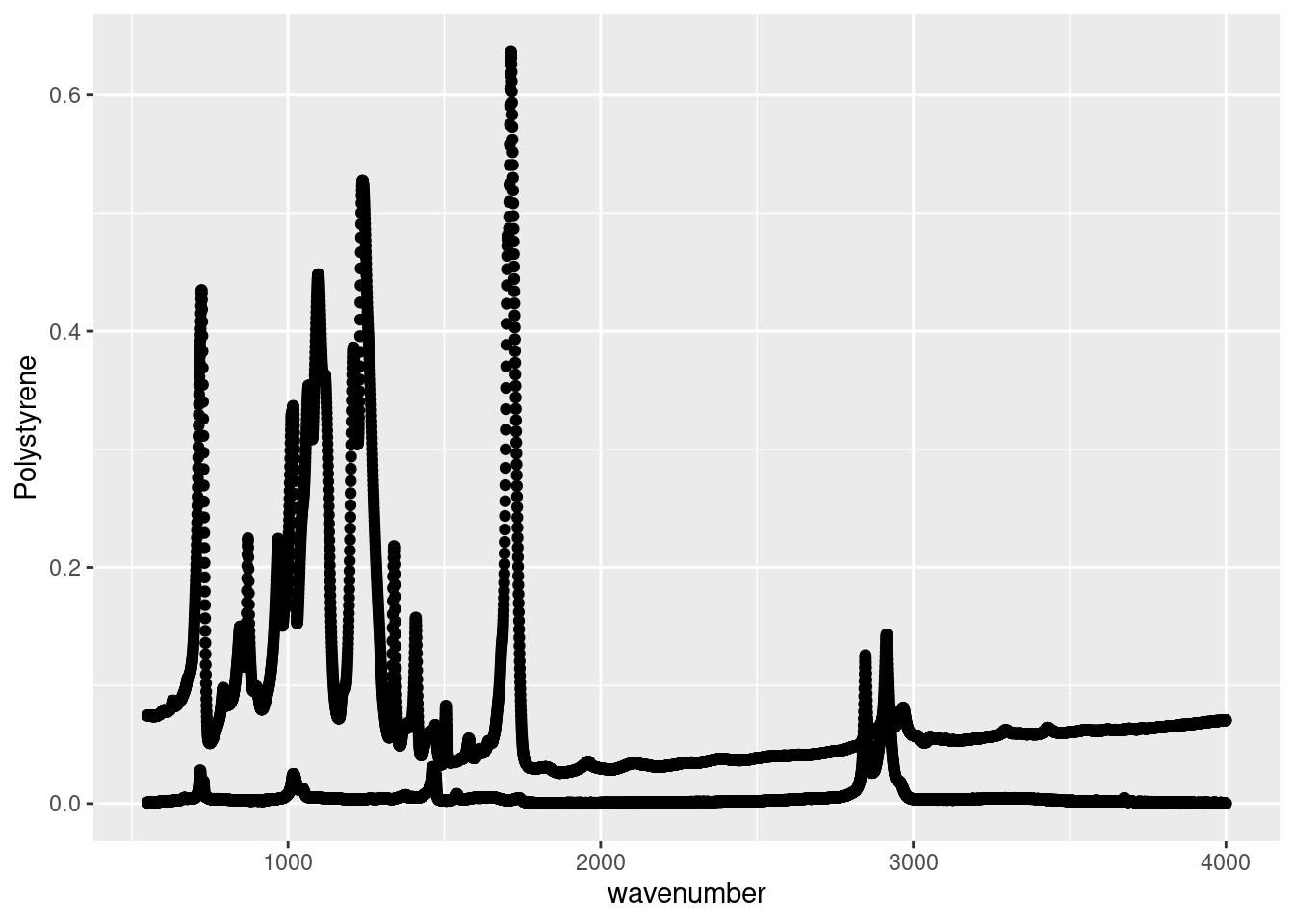

While the code above works, it’s not particularly handy and undermines much of the utility of ggplot.

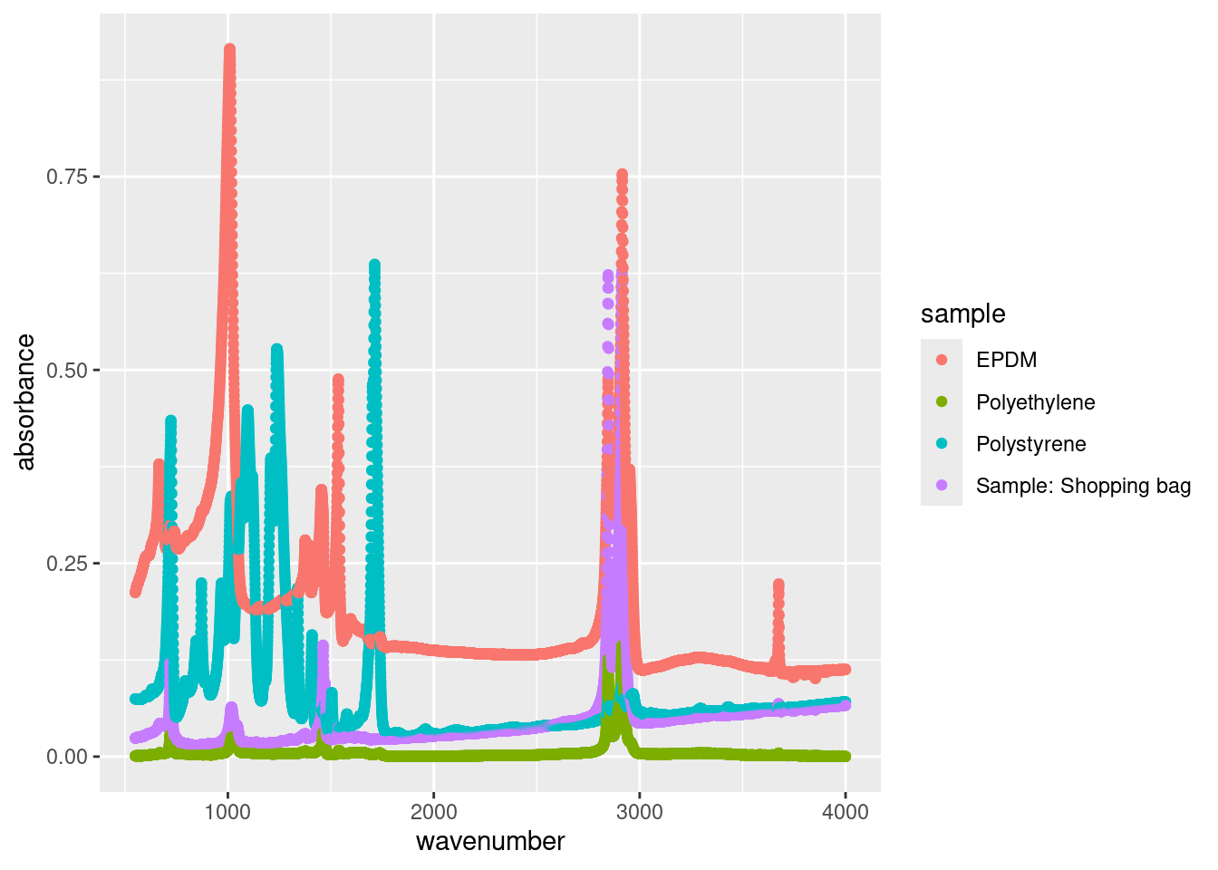
On the other hand, the long format will better work to show all 4 materials’ absorbance and wavenumber scatterplot in one graph without having to repeat the ggplot call.

ggplot(data = atr_plastics, 
       aes(x = wavenumber, 
           y = absorbance, 
           colour = sample)
       ) +
  geom_point()

15.2 Making Data Longer

Now that we learned the difference between long and wide formats, how did we actually transform the original wide format ATR plastic data into the longer format?

We transformed the original wide format data into a longer format using pivot_longer() function. This function reshapes the data by stacking or melting multiple columns into a single column, making it easier to work with and analyze. By specifying the appropriate arguments such as cols, names_to, and values_to, we can control how the data is reshaped.

Let’s look at the following code.

# Transform the original (wide) data into long format
atr_long <- pivot_longer(atr_plastics_wide, cols = -wavenumber, 
               names_to = "sample",
               values_to = "absorbance")

DT::datatable(head(atr_long, 50))

Let’s break down the code we’ve executed via the pivot_longer function:

cols = -wavenumber specifies that we’re selecting every other column but wave number.
- we could have just as easily specified each column individually using cols = c("EPDM",...) but it’s easier to use - to specify what we don’t want to select.
names_to = "sample" specifies that the column header (i.e. names) be converted into an observation under the sample column.
values_to = "absorbance" specifies that the absorbance values under each of the selected headers be placed into the absorbance column.

Beyond what we showed here, pivot_longer has many other features that you can take advantage of. For more details and the possibilities of this function you can read the examples listed on the pivot_longer page of the tidyverse.

15.3 Making Data Wider

How about making a data wider? We can utilize pivot_wider function.

Essentially, pivot_wider is used to spread key-value pairs across a dataset, transforming it from a long to a wide format. This is especially useful when you need your data structured in a wide matrix for certain analytical procedures or visual presentations.

The subsequent code utilizes the pivot_wider function to convert the long format data (atr_long) back into the original wider format. Here, names_from specifies the column containing the variable names, and values_from specifies the column containing the variable values. Running head(atr_wide) allows us to inspect the first few rows of the resulting wider format data, confirming that the transformation successfully reverted the data to its original structure.

# Transform the long format data back into the wider format (= original data)
atr_wide <- pivot_wider(atr_long, 
                        names_from = sample, 
                        values_from = absorbance)

head(atr_wide)

## # A tibble: 6 × 5
##   wavenumber  EPDM Polystyrene Polyethylene Sample..Shopping.bag
##        <dbl> <dbl>       <dbl>        <dbl>                <dbl>
## 1       550. 0.212      0.0746     0.000873               0.0236
## 2       551. 0.212      0.0746     0.000834               0.0238
## 3       551. 0.213      0.0745     0.000819               0.0239
## 4       552. 0.213      0.0745     0.000825               0.0239
## 5       552. 0.214      0.0745     0.000868               0.0240
## 6       553. 0.214      0.0746     0.000949               0.0240

Here’s a breakdown of this code:

names_from = sample: This argument specifies which column in our long data will be used to create new column headers in the wide format. Each unique value in the sample column becomes a separate column in the resulting wide dataset.
values_from = absorbance: This tells R that the values filling these new sample columns should be taken from the absorbance column.

The result is a more traditional, wide-format dataset where each column represents a different sample’s absorbance values, facilitating side-by-side comparisons.

The pivot_wider function is not only useful for converting long data to wide but also for data summarization and creating formats suitable for reports or specific analyses. If you’re dealing with summarized data, such as averages or counts, spreading this data into a wide format can make it more interpretable and easier to analyze.

Furthermore, pivot_wider can be an essential part of a more complex data transformation process. In many cases, data manipulation might require alternating between widening and lengthening to achieve the desired structure for your analysis.

To learn more about the pivot_wider function, we recommend reading the documentation here.

15.4 Summary

In summary, the relationship between wide and long data formats in R is inverse, meaning that transforming data from one format to the other and back again using functions like pivot_longer() and pivot_wider() is straightforward and reversible. This flexibility allows researchers to choose the most suitable format for their analysis needs. In general, the decision to use wide or long format depends on the specific characteristics of the data and the analytical tasks at hand. Here’s a recap of when to use each format:

Use wide format when:
- Each variable has its own column.
- Observations are in rows, and variables are in columns.
- The data is more compact and intuitive for viewing multiple variables simultaneously.
Use long format when:
- Multiple variables are stored in the same column.
- Each row represents a unique observation or measurement.
- The data is conducive to statistical analysis and visualization, especially when dealing with repeated measures or categorical variables.

Understanding both pivot_longer and pivot_wider equips you with a versatile toolkit for shaping your data. Whether you’re preparing data for specific package requirements, like matrixStats or matrixTests, or simply need to restructure your dataset for clarity and analysis, these functions are invaluable in the R programming environment.

By understanding the inverse relationship between wide and long data formats and knowing when to use each format, we can also effectively manage and analyze our data to derive meaningful insights and conclusions.

15.5 Further reading

As always, the R for Data Science book goes into more detail on all of the elements discussed above. For the material covered here you may want to read Chapter 12: Tidy Data.

15.6 Exercise

There is a set of exercises available for this chapter!

Not sure how to access and work on the exercise Rmd files?

Refer to Running Tests for Your Exercises for step-by-step instructions on accessing the exercises and working within the UofT JupyterHub’s RStudio environment.
Alternatively, if you’d like to simply access the individual files, you can download them directly from this repository.

Always remember to save your progress regularly and consult the textbook’s guidelines for submitting your completed exercises.