Chapter 11 Tidying Your Data
You might not have explicitly thought about how you store your data, whether working in Excel or elsewhere. Data is data after all. But having your data organized in a systematic manner that is conducive to your goal is paramount for working not only with R, but all of your experimental data. This chapter will introduce the concept of tidy data, and how to use some of the tools in the dplyr package to get there. Lastly we’ll offer some tips for how you should record your data in the lab. A bit of foresight and consistency can eliminate hours of tedious work down the line.
11.1 What is tidy data?
Tidy data has “…each variable in a column, and each observation in a row…” (Hadley Wickham 2014) This may seem obvious to you, but let’s consider how data is often recorded in lab, as exemplified in Figure 11.1A. Here the instrument response of two chemicals (A and B) for two samples (blank and unknown) are recorded. Note how the samples are on each row and the chemical are columns. However, someone else may record the same data differently as shown in Figure 11.1B, with the samples occupying distinct columns, and the chemicals in rows. Either layout may work well, but analyzing both would require re-tooling your approach. This is where the concept of tidy data comes into play. By reclassifying our data into observations and variables we can restructure our data into a common format: the tidy format (Figure 11.1C).
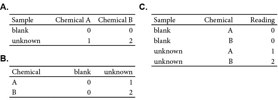
Figure 11.1: (A and B) The same data in different formats. (C) The data organized with clear variables and observations.
Organizing data into distinct variables (like Sample, Chemical, and Reading) enhances clarity. This reorganization doesn’t change the data but rearranges it for better compatibility with analytical tools.
11.2 Tools to tidy your data
Now one of the more laborious parts of data science is tidying your data. If you can, follow the tips in the Tips for recording data section, but the truth is you often won’t have control. To this end, the tidyverse offers several tools, notable dplyr (pronounces “dee-plier”), to help you get there.
Let’s revisit our spectroscopy data from the previous chapter, but in a slightly different format. We will learn a variety of tools to change the format of a dataset as we move through Part 3 of this resource, but for now just observe some of the changes we make to the ATR plastics data in comparison to what we did in the previous chapter.
As we can see this our ATR spectroscopy results of several plastics, as recorded for a CHM 317 lab, is structured similarly to the example in Figure 11.1A. The ATR absorbance spectra of the four plastics are recorded in separate columns. Again, this format makes intuitive sense when recording in the lab, and for working in Excel, but isn’t the friendliest with R. When making plots with ggplot, we can only specify one y variable. In the example plot below it’s the absorbance spectrum of Polystyrene. However, if we wanted to plot the other spectra for comparison, we’d need to repeat our geom_point call. In Ggplot Basic Visualizations after we’ve tidied this data we will see how easily we can make more interesting and informative plots with the data in this new format.
# Plotting Polystyrene absorbance spectra
ggplot(data = atr_plastics,
       aes(x = wavenumber,
           y = Polystyrene)) +
  geom_point()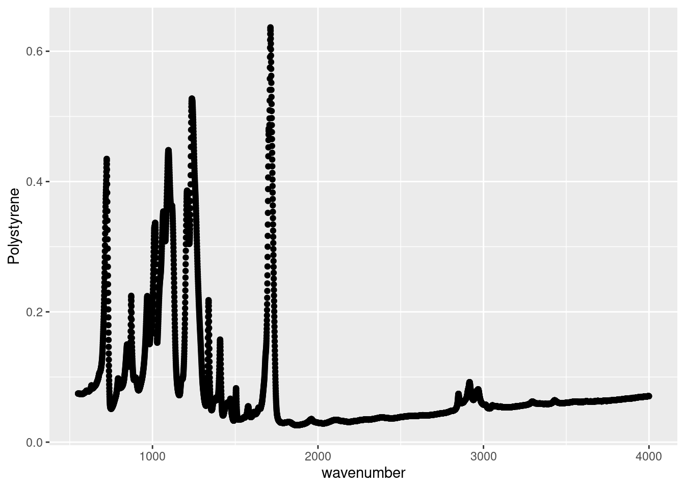
# Plotting Polystyrene and Polyethylene absorbance spectra
ggplot(data = atr_plastics,
       aes(x = wavenumber,
           y = Polystyrene)) +
  geom_point() +
  geom_point(data = atr_plastics,
             aes(x = wavenumber,
                 y = Polyethylene))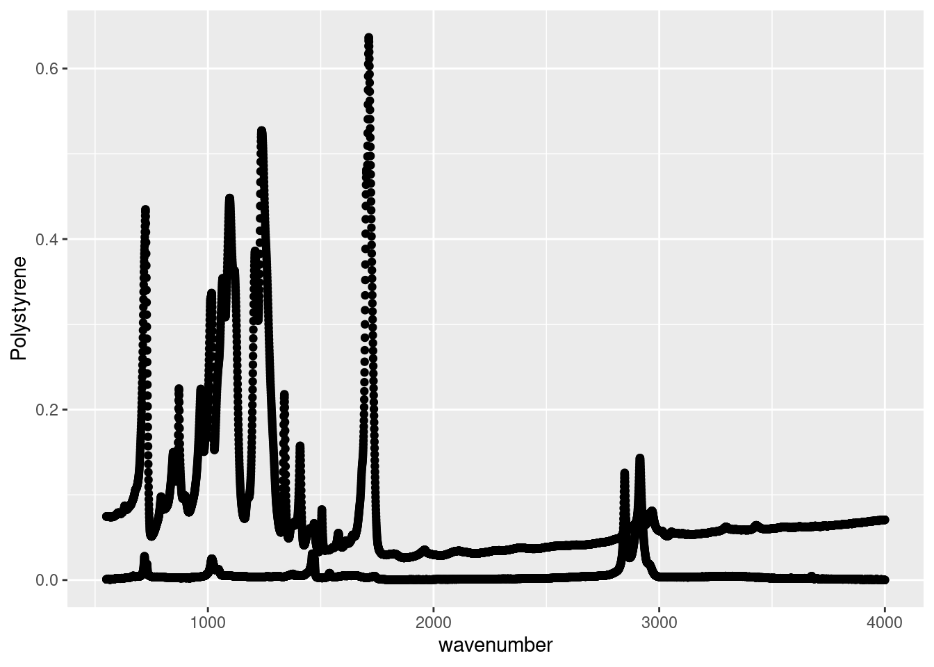
11.2.1 Selection helpers
There are multiple ways to select columns and variables with the dplyr package. For a complete rundown of other useful helper functions please see Subset columns using their names and types. starts_with() for selecting columns from a prefix, and contains() for selecting columns that contain a string are two of the most useful.
11.2.2 Separating columns
Sometimes your data has already been recorded in a tidy-ish fashion, but there may be multiple observations recorded under one apparent variable, something like 1 mM for concentration. As it stands we cannot easily access the numerical value in the concentration recording because R will encode this as a string due to the mM. We can separate data like this using the separate function.
Consider the following example scenario. You have sample names you’ll pass along to your TA where you crammed as much information as possible into that name so you and your TAs know exactly what’s being analyzed. In this example, the sample name contains the location (Toronto), the chemical measured (O3 or NO2) and the replicate number (i.e. 1).
# Example with multiple encoded observations
sep_example <- data.frame("sample" = c("Toronto_O3_1","Toronto_O3_2", "Toronto_NO2_1"),
                          "reading" = c("10", "22", "30"))
sep_example
## sample reading
## 1 Toronto_O3_1 10
## 2 Toronto_O3_2 22
## 3 Toronto_NO2_1 30Using the separate function we can split up these three observations so we can properly group our data later on in our analysis.
# Separating observations
separated_data <- separate(
    sep_example,
    col = sample,
    into = c("location", "chemical", "replicateNum"),
    sep = "_",
    convert = TRUE)

separated_data
## location chemical replicateNum reading
## 1 Toronto O3 1 10
## 2 Toronto O3 2 22
## 3 Toronto NO2 1 30Let’s break down what we did with the separate function:
- The first input,
sep_example, is the data frame that we’re operating on. col = samplespecifies we’re selecting thesamplecolumn.into = c(...)specifies what columns we’re separating our name into.sep = "_"specifies that each element is separated by an underscore (_).convert = TRUEconverts the new columns to the appropriate data format. In the original column, the replicate number is a character value because it’s part of a string,convertensures that it’ll be converted to a numerical value.
11.2.3 Uniting/combining columns
The opposite of the separate function is the unite function. You’ll use it far less often, but you should be aware of it as it may come in handy. You can use it for combining strings together, or prettying up tables for publication/presentations as shown in Summarizing Data.
# Uniting observations
united_data <- unite(separated_data,
                     col=sample_reunited,
                     c("location", "chemical", "replicateNum"),
                     sep = "_",
                     remove = TRUE)

united_data
## sample_reunited reading
## 1 Toronto_O3_1 10
## 2 Toronto_O3_2 22
## 3 Toronto_NO2_1 30You can read more about the unite function here.
11.2.4 Renaming columns/headers
Sometimes a name is lengthy, or cumbersome to work with in R. While something like This_is_a_valid_header is valid and compatible with R and tidyverse functions, you may want to change it to make it easier to work with (i.e. less typing).
First, here’s an example with some awkward column names:
bad_col_names <- data.frame("UVVis_Wave_Length_nM" = c(500, 501),
                            "Absorbance" = c(1, 0.999))

colnames(bad_col_names)
## [1] "UVVis_Wave_Length_nM" "Absorbance"Use rename() to change the column name and save the result to a new data frame:
renamed_data <- rename(bad_col_names, wavelength_nM = UVVis_Wave_Length_nM)

# Inspect the column names of the renamed data frame
colnames(renamed_data)
## [1] "wavelength_nM" "Absorbance"11.2.5 Chaining multiple operations
So far we learned some standalone functions that can tidy up your data. But what if you want to do multiple of these operations to a dataset?
Let’s start by talking about the seemingly intuitive but tedious approach. We can transform data by breaking down the process into individual steps:
selected_data <- select(atr_plastics, wavenumber, EPDM, `Sample: Shopping bag`)
atr_plastics_transformed <- rename(selected_data, Wave_Num = wavenumber)

atr_plastics_transformed
## # A tibble: 7,157 × 3
## Wave_Num EPDM `Sample: Shopping bag`
## <dbl> <dbl> <dbl>
## 1 550. 0.212 0.0236
## 2 551. 0.212 0.0238
## 3 551. 0.213 0.0239
## 4 552. 0.213 0.0239
## 5 552. 0.214 0.0240
## 6 553. 0.214 0.0240
## 7 553. 0.215 0.0241
## 8 553. 0.215 0.0241
## 9 554. 0.216 0.0242
## 10 554. 0.216 0.0242
## # ℹ 7,147 more rowsNow, let’s see how we can transform the same atr_plastics tibble using the %>% operator by chaining operations.
atr_plastics_transformed <- atr_plastics %>%
    select(wavenumber, EPDM, `Sample: Shopping bag`) %>%
    rename(Wave_Num = wavenumber)

atr_plastics_transformed
## # A tibble: 7,157 × 3
## Wave_Num EPDM `Sample: Shopping bag`
## <dbl> <dbl> <dbl>
## 1 550. 0.212 0.0236
## 2 551. 0.212 0.0238
## 3 551. 0.213 0.0239
## 4 552. 0.213 0.0239
## 5 552. 0.214 0.0240
## 6 553. 0.214 0.0240
## 7 553. 0.215 0.0241
## 8 553. 0.215 0.0241
## 9 554. 0.216 0.0242
## 10 554. 0.216 0.0242
## # ℹ 7,147 more rowsWe will formally introduce the unfamiliar operator %>% (pipe) in the next chapter The Pipe: Chaining Functions Together. For now, just remember that there is a way to chain your functions like the above example!
11.3 Tips for recording data
In case you haven’t picked up on it, tidying data in R is much easier if the data is recorded consistently. You can’t always control how your data will look, but in the event that you can (i.e. your inputting the instrument readings into Excel on the bench top) here are some tips to make your life easier:
- Be consistent. If you’re naming your samples make sure they all contain the same elements in the same order. The sample names
Toronto_O3_1andToronto_O3_2can easily be broken up as demonstrated in Separating columns;O3_Toronto_1,TorontoO32, andToronto_1can’t be. - Use as simple as possible headers. Often you’ll be pasting instrument readings into one
.csvusing Excel on whatever computer records the instrument readings. In these situations it’s often much easier to paste things in columns. We will learn more about how to do this in the next chapter. - Make sure data types are consistent within a column. This harks back to the Importing your data into R chapter, but a single non-numeric character can cause R to misinterpret an entire column leading to headaches down the line.
- Save your data in UTF-8 format. Excel and other programs often allow you to export your data in a variety of
.csvencodings, but this can affect how R reads when importing your data. Make sure you selectUTF-8encoding when exporting your data.
11.4 Further reading
As always, the R for Data Science book goes into more detail on all of the elements discussed above. Topics covered here are explored in more detail in Chapter 12: Tidy Data.
11.6 Exercise
There is a set of exercises available for this chapter!
Not sure how to access and work on the exercise Rmd files?
Refer to Running Tests for Your Exercises for step-by-step instructions on accessing the exercises and working within the UofT JupyterHub’s RStudio environment.
Alternatively, if you’d like to simply access the individual files, you can download them directly from this repository.
Always remember to save your progress regularly and consult the textbook’s guidelines for submitting your completed exercises.